Wednesday, April 15, 2015
CHF loses to RMSprop
This is a Technical Report of interest mostly to folks who play with neural nets, especially in an online setting where batch methods are difficult. Most everyone else can safely skip this without regret. :)
This is just a quick report, suitable perhaps for the Journal of Negative Results, of some experiments with various learning/optimizing algorithms run on the same underlying function. In this case, I just ended up using example #4 (multi-layer neural net on MNIST data using cross-entropy cost) from a theano tutorial as a base, since it was easy to swap other code in for the RMSprop implementation they used in the example. All tests were run on the same network with the same data, so all I'm testing here are different ways to follow the gradient.
I was not very diligent in doing the runs, in the sense that I didn't really try a wide range of tuning parameters and whatnot to make sure I was doing a fair comparison, but that was semi-intentional: I am most interested in finding an algorithm that just works without fuss, because when I'm doing actual experiments (on different architectures or whatnot) I don't want to wonder whether the experiment failed because the architecture is bad or because I was way off on my tuning parameters. Ick.
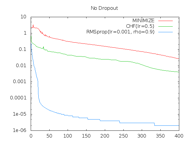
The executive summary of the result is: RMSprop beat everything under all conditions. This is a little disappointing because RMSprop does require hand tuning; but it's not as bad as it might seem as I will explain below (with some ideas for how to make an architecture a good RMSprop candidate). For reference: all RMSprop does is scale each component of the gradient by the inverse of its recent geometric mean (over time) so that, roughly speaking, parameters move at a rate relative to the consistency of their gradient but insensitive to its magnitude.
I did not try a bona fide Hessian Free algorithm, so if someone sees an easy way to plug the above example into their spiffy HF code, I'd love to see the resulting plot.
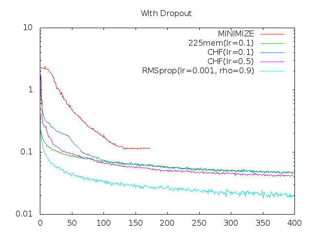
Here are my results. The X axis is the number of times through the full data set (epochs), and the Y is the mean value of the cost function for that epoch. For the moment I'm assuming regularization terms would be explicit so am not concerned with over-fitting:


The dropout version has random dropouts of input and hidden nodes per pattern. (See the code linked above for details.) I'm only showing the most representative or two runs of each here, so assume other parameter values did similar or worse in general.
Minimize is using minimize.py which "is a straightforward Python-translation of Carl Rasmussen's Matlab-function minimize.m". I fed it a full epoch for (a single invocation of) the cost function, and simply plotted the cost for the current parameter value each time minimize called the cost function.
The rest were done more in an SGD style, although I retained the example's 128-size mini-batches rather than going full online SGD.
RMSprop is vanilla as provided in the example code linked above.
23mem is sort of a hybrid of LeCun's method in No More Pesky Learning Rates and RMSprop, in that I replaced the Hessian in LeCun's method with simple RMS of the gradient (in both cases that is the scale-normalizing constant), resulting in a wince-worthy learning rate of mean(g)^2/mean(g^2)^1.5. I did not try LeCun's method as-is (again, curious to see the results if anyone does).
Comparing CHF (Continuous Hessian-Free) was the main reason I ran this experiment. CHF is an attempt to gain some of the advantages of the Hessian Free approach in an SGD context. My second attempt at CHF was to follow a (meta) gradient toward the solution of the vector that when multiplied by the Hessian results in the current raw gradient, and to follow that vector. That is, over time, it should "steer" in the direction (and magnitude) of the optimal Newton step. It did sort of work in early tests, but it felt too sensitive to noise and tuning, so I abandoned that and returned to my first attempt which proved more stable: Simply maintaining an estimate of the current gradient and Hessian*gradient product, and using their ratio as the traveling speed.
It is similar to a momentum-based approach in that the gradient estimate is based on a time-decayed average. However, because we have an estimate of the Hessian*gradient product, we can not only use that to set an "optimal" travel speed, but also to update the gradient estimate after each step as well, and thus get a true current estimate of the gradient as opposed to a lagging one. Specifically, if we are traveling at r times the optimal speed (for some r < 1), we can simply lop off r fraction of the gradient (because that's roughly how much we "use up" when we advance in the direction of the gradient by r fraction of a Newton step). This is in addition to the exponential-decay blend of the current estimate with the currently observed gradient. That is, rather than blend old gradient estimate with current gradient, we first bring the estimate forward to the current time, and then blend with the current (single pattern or mini-batch) gradient. This results in a smoothed gradient follower (like a momentum-based approach) that doesn't overshoot! In simpler tests it performed really well--on something like the banana function, it goes straight down the steep face, slows and turns as it nears the bottom, and heads down the trough to the target. This worked (though more slowly) even if I added substantial random noise to the gradient. (Iirc, it did better than RMSprop at the banana.) Too bad RMSprop beats it hands down on the more substantial tests.
The theano code is below, which is nearly plug-in swappable for the RMSprop method except that for CHF the parameters need to be consolidated into a single variable (x). In theory, lr can be set to 1.0, or maybe 0.9, as I borrowed LeCun's adaptive "memory size" to set the scale (relative to the Newton optimum) based on the ratio of gradient mean to noise. So, in theory, CHF is essentially free of tuning parameters. I've verified (not very rigorously) that it does track actual (as opposed to delayed) gradient pretty well. That trick might prove useful elsewhere some day.
def CHF(cost, x, lr=0.1):

    g = T.grad(cost=cost, wrt=x)

    mem = theano.shared(100.)

    r   = 1./mem
    rn  = 1.-r

    mG  = theano.shared(x.get_value() * 0.)
    mG2 = theano.shared(x.get_value() * 0.)
    mHg = theano.shared(x.get_value() * 0.)

    mG_  = rn*mG  + r*g
    mG2_ = rn*mG2 + r*g*g
    mHg_ = rn*mHg + r*T.Rop(g, x, mG_)           # Rop(g, x, mG) = Hessian*mG

    gg = mG_.dot(mG_)
    l_ = gg/(abs(mG_.dot(mHg_)) + 0.00000001)

    return [
        (x, x - r*l_*mG_),
        (mG, mG_ * rn),
        (mHg, mHg_ * rn),
        (mG2, mG2_ * rn),
        (mem, 1. + mem*(1. - lr*gg/T.sum(mG2_))),
        ]
Again, this is mostly a "negative result" since RMSprop does better, but there might be some useful ideas in it. And, sorry, I realize theano is awfully cryptic even if you have used it and nearly opaque if you haven't. I'm assuming nobody actually cares the details of CHF but if you do just email me and I'll be happy to clarify.
Now, some thoughts on the above results, and why RMSprop works well:
Minimize failed on the dropout case because it presupposes a static landscape and the dropout code changes the effective cost function every call. No surprise there; I was more surprised it worked at all.
In either case, my best guess is that CHF and Minimize are both falling into local minima in some subset of the parameter space, and that CHF does better than minimize early on because it's more noisy before it has good gradient estimates. Run long enough, they may both wind their way down to over-fitting as well as RMSprop, but I'm guessing their relative stability is a cost rather than benefit in terms of convergence speed here.
CHF has a very one-track mind: It heads carefully (but at an optimal speed) in the direction of the strongest gradient. It avoids the high-curvature directions simply by aiming well enough to mostly stay in the bottom of the associated trough where the gradient is zero in that direction; and the no-overshooting trick allows it to do a tight bottom turn into the trough. The stair-steppy progress of CHF is indicative of such bottom turns.
RMSprop, by contrast, is pretty much working all the angles all the time. My sense of the implicit premise behind RMSprop is that the parameter values themselves all fall roughly within a common range. That is, rather than worrying about the scaling of the gradient space at all, we can think instead about the scaling of the parameter space itself: If our parameters are all somewhat on-par in terms of how sensitive they are across their on-par range, then it seems quite reasonable to move at roughly a constant speed in that space. Or put another way, if that premise holds, then we can infer that the gradient/hessian ratio should be very roughly constant everywhere. More usefully, we can design our architectures with that in mind, to make them as RMSprop-friendly as possible. Note that this is not the same as saying the gradient is the same everywhere--the gradient magnitudes could vary widely by parameter and by location in the parameter space. The premise is simply that those same variations will tend to be reflected in the Hessian as well.
It's probably safe to say that premise breaks down for deep nets (or at least for un-primed deep nets that aren't designed to be RMSprop friendly). But setting that aside...
One question is why does RMSprop seem to settle reasonably well, at least here, into a high-precision solution even in the absence of a decaying learning rate? I.e., if the parameter jumps are nearly of fixed size even when the mean gradient is nearly zero, why isn't it noisily bouncing all over the place under the microscope of 1e-6 cost deviations? One possible answer, which I suppose I could test if I weren't lazy, is that near a minimum, the many parameters essentially take up a binomial distribution around the center, bouncing back and forth at random (but by roughly the same amount), so that at any given moment they all cancel each other out. That is, the minimum error is still proportional to that minimum jump size (related tightly to our hand-specified learning rate), but with each parameter's momentary deviation mostly statistically uncorrelated with the rest, and so lacking any unified direction and hence any substantial cumulative effect.
If the depiction is accurate, presumably the same thing is going on in the higher-curvature directions when RMSprop is traveling down a trough, which simultaneously creates a sort of stability of the mean while also exploring the adjacent space for escapes. That is, rather than riding carefully down the bottom of the trough, perhaps it touches both sides in many places and rides the mean (the inferred trough bottom), which allows a quick turn if one of the trough sides falls away.
But whatever the reasons, it works. At least within the SGD context I will probably stick with RMSprop for now, with an eye toward keeping my parameter space uniform in scale and impact. (So much easier than trying to keep the gradient space uniform, which is what you would need to make an architecture vanilla-SGD friendly...)
[Update: I will likely add Adam to the above plots tomorrow.]