Sunday, June 29, 2008
Fusion-Reflection - Self-Supervised Learning
Thought I'd resurrect an old writeup for giggles and grins. This was never published (this version of the paper wasn't written to be published--it was written to be understood), but it made the rounds. Granger liked it. Hinton dismissed it. Compare the network under Learning Context to Numenta's patented algorithms... [Also available in black on white.]
Fusion-Reflection
Self-Supervised Learning
Simon Funk
May, 1993
Abstract
By analyzing learning from the perspective of knowledge acquisition, a number of common limitations are overcome. Modeling efficacy is proposed as an empirical measure of knowledge, providing a concrete, mathematical means of "acquiring knowledge" via gradient ascent. A specific network architecture is described, a hierarchical analog of node-labeled Hidden Markov Models, and its evaluation and learning laws are derived. In empirical studies using a hand-printed character recognition task, an unsupervised network was able to discover n-gram statistics from groups of letter images, and to use these statistics to enhance its ability to later identify individual letters.
Introduction
In the pursuit of synthetic intelligence, the study of learning is of central importance. Many tasks which seem simple to us in fact require a vast hierarchy of knowledge. Consider the task of identifying a pictured animal: this first requires an implicit understanding of more fundamental concepts such as visual continuity, edges, orientation, depth, form, and the nature of identity itself--just to name a few. Not only does this represent a vast amount of knowledge, but our own understanding of some of the crucial concepts is still incomplete. Ideally, the study of learning will produce an adaptive intelligence that can discover these principles on its own, and perhaps even reveal them to us, rather than vice-versa.
For an intelligent system to be capable of learning, aspects of its behavior must be modifiable. We can imagine the system as a black box with input, output, and set of modifiable, internal variables, or free parameters. These internal parameters determine the behavior of the box and can be envisioned as a set of controlling dials. Inside the box is some fixed algorithm, the evaluation law, which combines the input with the state of the dials to generate output. It is presumed that this algorithm is sufficiently robust that some configuration of the dials will produce the desired behavior. The goal of the learning law is to find this configuration.
Consider, for instance, the name-that-animal problem. Upon unpacking our newly arrived ACME All-Purpose Black Box, we find its dials in a random configuration. After hooking a scanner to the box's input and a printer to its output, we observe the expected: the box does no better than chance. In fact, it does worse, outputting "blblblblbl"--which is not an animal at all. How do we determine the configuration of dials that will make the box name-that-animal?
The most direct approach is simply to compute the proper configuration, and set the dials. Doing this, however, requires an analytic solution to the particular evaluation law in question. Suppose, for example, we wish the box to light a bulb when it sees the word "idea". If the box had four dials with settings from "a" to "z", we could simply dial in i-d-e-a, and we would be done. On the other hand, if the evaluation law processed the input through some complex equation involving the dial settings, then there may be no straightforward, one-step method of determining a good configuration. In practice, the most flexible evaluation laws fall into the latter category, having no known analytic solutions.
When the solution is not analytically attainable, we can attempt to incrementally improve performance instead. This basic technique is known as hill climbing or gradient ascent, for reasons which the following example should make clear: Consider a two-dial box that we wish to configure to perform some task, such as lighting a bulb when it sees a cow. For any particular configuration of the dials, the box will have some measurable performance. In this case, the average brightness of the bulb when it sees a cow minus that when it doesn't would serve as a good measure of performance--it is least when the box is performing badly, and greatest when, and only when, the box is performing perfectly. These three values together, the two dial settings and the measure of performance, can be used to define a topological map, where the dials define the x,y location and the corresponding performance defines the altitude. Finding the optimal configuration amounts to locating the highest peak on the map. For all but the most trivial problems, an exhaustive search--computing the performance at every point on the map--is computationally out of the question. Instead, we can start at a random location and, by computing the direction of slope (the gradient), simply travel uphill until we reach a peak. This is much like hiking to the top of an unexplored mountain while blindfolded--the best we can do is to walk uphill and hope that the first peak we find is the highest one (or at least high enough to meet our needs). The same technique applies regardless of the number of free parameters (dials), though the hill analogy is difficult to visualize in the higher dimensional spaces.
In order to perform gradient ascent, we need a concrete measure of the system's performance; the most direct method is to compare its output against desired output. For instance, in the name-that-animal problem, the natural measure of performance would be the percentage of correctly named animals. Supervised algorithms--algorithms which learn from examples of correct answers--are generally measured this way, by comparing their answers against the given examples. Gradient ascent using this measure of performance means finding those incremental changes to the free parameters that will bring the system's output ever closer to the desired output.
For many real-world problems, however, this kind of performance measure is insufficient as a learning guide. The assumption is made, when hill climbing, that there will be a slope to follow, that at each step there will be some incremental change of the parameters that can improve performance. What if the problem is so difficult that this is not true? Consider again the problem of lighting a bulb when the input image represents a cow. From an initial random configuration, the system has no concept of spatial continuity, edges, or orientation--let alone of cow-ness. A great deal of knowledge must be acquired before the system can even begin to improve its cow- identifying ability. If improving that ability is its only guide to learning, then it has no guidance in acquiring the prerequisite knowledge. Returning to the hill climbing analogy: as the problem becomes more difficult, the performance surface looks less and less like the smooth hill we would like to imagine, and begins to look more like Pinnacles National Park--a vast plane with narrow spikes jutting up here and there. Imagine trying to find the highest peak there while blindfolded.
As a possible way around this problem, instead of measuring the final output performance, we could measure the performance at each successive stage of abstraction. For instance, rather than having a single black box solve the cow-light problem in one big step, we could cascade a number of boxes end-to-end, the first receiving the picture and the last lighting the bulb. Then we might train the first to abstract edges from the picture, the next to abstract curves from the edges, then shape from the curves, form from the shape, and finally cow-ness from the form. Our hope would be that each of these smaller problems would be simple enough to solve with gradient ascent. Unfortunately, predetermining the various stages of abstraction presumes considerable knowledge of the final solution. If we had that, we probably wouldn't need an adaptive algorithm at all.
Instead of predetermining the stages of abstraction, we could supply an algorithm to discover these stages on its own. Many unsupervised learning laws--which do not receive output examples--use an algorithmic measure of performance to abstract "useful" features from their input. Imagine a series of boxes, each ideally containing the same algorithm, and each learning to perform a single stage of abstraction on its input. The algorithm may, for example, form categories based on groupings of similar input patterns and convey those categories to the next stage. Using this approach, a box receiving images of handwritten characters might form a unique category for each letter of the alphabet and pass these categorized letters to the next box, which might form a unique category for each word, and so on.
What kind of final output could we expect from such a system, where each stage of abstraction is guided only by a local measure of performance? It is hard to say. Having eliminated the global measure of performance in favor of the more easily solved local measures, the system is left with no overall goal. Each stage abstracts certain features and sends them onward, without ever receiving feedback as to how globally valuable those features are. They may be useless, and more importantly, crucial features may be ignored altogether. For instance, the box categorizing letters may not realize that O and Q need to be differentiated, since they are visually similar. Conversely, it may form multiple categories for a letter like A, which can be drawn in more than one way. Resolving ambiguities like this without feedback is impossible--the necessary information is simply unavailable.
Fusion-Reflection
To advance learning beyond these limitations, we need a global measure of the process of abstraction--a measure of the system's knowledge as a whole. When we considered only the final output performance, we ignored the earlier stages of abstraction; on the other hand, when we considered only a single stage at a time, we ignored the need to coordinate abstraction from a global perspective. Measuring the system's total knowledge would solve both of these problems. Even the earliest stages of abstraction represent knowledge, so a system using knowledge as its measure of performance has guidance from the ground up. Likewise, such a system must coordinate abstraction from a global perspective, since (as in the letters example above) certain knowledge may not become available until higher-level knowledge has been learned. In terms of gradient ascent, using knowledge as our performance measure should define a gradient topology that is easily traversed from beginning to end by normal hill climbing.
But how do we measure "knowledge"? This might seem a difficult problem, but fortunately, an empirical measure of knowledge exists in the system's ability to model its input--that is, its ability to generate patterns similar in nature to the input patterns. Specifically, if the system could, from scratch, generate "imaginary" examples of input patterns with exactly the same probability with which those patterns would actually occur, then the system can be said to have a complete working knowledge of the input. Consider a black box whose input is a camera which takes random snapshots of everyday life on earth. If that box could in turn fabricate imaginary pictures of life on earth in exactly the same probabilistic distribution as they would actually occur, then it must contain all relevant knowledge about life on earth. Every picture would implicitly convey the laws of physics--ropes would hang in catenaries, objects would rest on supporting surfaces, and frisbees would frequently be underneath cars. Every human emotion would be understood--the child walking a fence would look amused, while the woman watching her child would look distraught. It would be safe to deduce that every aspect of visible existence must in some way be encoded in that box, whether by brute force as a catalog of all possible pictures, or by abstraction as the fundamental laws of nature.
The key point is that a model does not record and playback like a VCR; it learns, then imagines things it has never seen before. And unlike the previously described systems, which produced as output some sort of analysis of a specific input, a model generates patterns from scratch--from the knowledge it has acquired about the general nature of its input.
Notice that the processes of observing (taking input) and acting (producing output) have become separate functions. We have shifted the focus from training the system to do a particular thing--performance enhancement--to having it simply learn about its input--knowledge acquisition. As such, the metaphor is no longer a black box with input and output, but rather a black box with input only. This input is, in essence, the box's window to the world--everything it needs to know is available in the input. The "desired output" of a supervised system becomes simply more input to the model--learning that the caption "cow" goes with the picture of a cow is no different from learning that this kind of leg belongs on a sheep, and that kind of leg belongs on a table.
In fact, since our goal is to acquire knowledge, we need not generate "output" patterns at all. Modeling efficacy is merely our measure of knowledge, not the ultimate goal. A model's output neither represents any transformation of the input, nor is it the desired end--it is simply proof of the model's knowledge. Applying that knowledge (as in pattern classification, pattern completion, etc...) is a separate problem and can be dealt with at a later time. (Fortunately, the structure required to obtain knowledge by modeling is generally useful in applying that knowledge as well. An example of this is provided in the specific treatment of Furf-I, the algorithm presented later in this paper.)
As an illustration of the modeling approach, consider the basic two-input Boolean logic functions (AND, OR, XOR, etc...). Traditionally, these are viewed as mapping functions, taking two inputs and producing a single output. From that perspective, the following tables are definitive:
                       AND                 OR                  XOR
                   x   y |    z      x    y |   z          x   y |   z
                   ------+-----      -------+----          ------+----
                   F   F |    F      F    F |   F          F   F |   F
                   F   T |    F      F    T |   T          F   T |   T
                   T   F |    F      T    F |   T          T   F |   T
                   T   T |    T      T    T |   T          T   T |   F
These tables specify, for a given function, how to map a given input (x,y) to its corresponding output (z). A model, on the other hand, makes no distinction between input and output. Instead, once trained, it generates each possible aggregate pattern (x,y,z) with some defined probability:
                        AND                    OR                         XOR
               x   y   z |     P      x   y   z |    P          x    y   z |     P
               ----------+-------     ----------+------         -----------+-------
               F   F   F |    30%     F   F   F |   30%         F    F   F |    30%
               F   T   F |    20%     F   T   F |    0%         F    T   F |     0%
               T   F   F |    15%     T   F   F |    0%         T    F   F |     0%
               T   T   F |     0%     T   T   F |    0%         T    T   F |    35%
               F   F   T |     0%     F   F   T |    0%         F    F   T |     0%
               F   T   T |     0%     F   T   T |   20%         F    T   T |    20%
               T   F   T |     0%     T   F   T |   15%         T    F   T |    15%
               T   T   T |    35%     T   T   T |   35%         T    T   T |     0%
Notice that these tables, although not directly specifying an input-output mapping, do contain all the necessary information to perform such a mapping. Further, these tables contain information about the relative frequencies of the patterns--information which the mapping tables could not convey. For example, if the OR model generates a pattern with y,z both true, then we can compute a 64% probability that x is also true. (Performing these computations does not necessarily require an exhaustive look-up table as we have here. See the Furf-I evaluation laws, below.)
Designing a Model
In order to use modeling efficacy as our measure of system performance, the system must first be a stochastic pattern generator. It is here, in designing the method of pattern generation, that we set the limits on the model's ability to learn: If a model cannot easily generate a particular pattern, then it cannot easily learn that pattern, since learning in this case is "learning to generate". Since the model is generating new patterns from scratch, its methods must be stochastic, or it would always generate the same thing. For example, consider a system that models biased coin tosses. Each time we ask the system to generate a pattern, it should randomly select heads or tails according to the bias of the coin being modeled. In this way, the system will behave just like the coin, turning up heads sometimes, tails others. Or, imagine a system that models snowflakes. The free parameters here could define the branching probabilities in a fractal algorithm--each newly generated snowflake would potentially be unique.
Training an adaptive system requires finding the gradient of the performance measure. In this case, the performance measure is modeling efficacy, which, in practical terms, can be measured as the probability that the model would have generated the training set (the set of patterns the model is given to learn from). Consider the biased-coin model again. To create a training set, we could flip the real coin four times, which might, for example, produce H-H-T-H. The probability of our model generating that training set is B3(1-B), where B is the model's bias for turning up heads. The gradient of this function is 3B2-4B3, which is positive when B<.75, negative when B>.75, and zero when B=.75. So, as we would expect, the gradient leads us to choose a bias of .75, which best represents the training set.
The next section describes a particular modeling architecture, Furf-I. The following sections derive the corresponding evaluation and learning laws. It is important to remember that these derivations are based on the method of pattern generation--so a firm understanding of the generation algorithm is an absolute prerequisite to understanding the evaluation and learning laws which follow.
Furf Nets
A Furf-I network is organized as a hierarchy of groups of nodes, where each node belongs to one and only one group. Connections can be made between any two nodes from different groups. Typically, however, connections are made at the group level, where all nodes in one group are fully interconnected to all nodes in another group. In the following illustrations, a connection shown between two groups indicates full nodal interconnection:
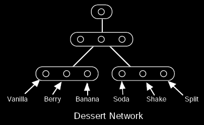
The network operates as a stochastic pattern generator from the top down. Pattern generation always begins by selecting the single node in the topmost group. Each connection downward from a selected node to a node below dictates the probability of selecting that lower node. Using these probabilities, a single node from each group below is randomly selected. Since only one node is selected from each group, the nodes within a group represent mutually exclusive possibilities. This process continues downward from each newly selected node until the bottom is reached. The resulting state of the bottom layer defines the generated pattern:
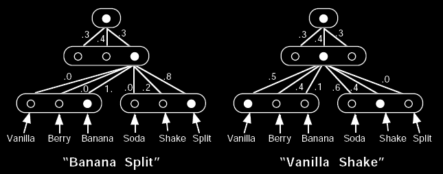
The evaluation law for a Furf network is a two-pass algorithm consisting of an upward and a downward pass. The upward evaluation law computes the probability that any particular node would generate a given pattern. For instance, from the dessert network example above, the upward evaluation law could tell us the probability that the middle node, of the middle group, would generate "Vanilla Shake" (in this case, 20%). Since the top-most node originates all generated patterns, the overall probability of the network generating a given pattern can be computed by applying the upward evaluation law to that top-most node. For example, the dessert network would, as a whole, generate "Vanilla Shake" with at least an 8% probability (or more, depending on the probabilities associated with the left-most node in the middle group).
The downward evaluation law computes the probability that any particular node was selected during the generation of a given pattern. This is useful for both pattern completion and categorization. For example, we can present the partial pattern "? Split" to the dessert network above by setting the Vanilla, Berry, and Banana nodes as equally likely, while setting the Split node to 1, and the Soda and Shake nodes to 0. After upward/downward evaluation, the Vanilla and Berry nodes would have a probability of 0, while the Banana node would have a probability of 100%, thus completing the pattern as "Banana Split". In general, however, the completed pattern will not be so definite. The pattern "? Shake", for instance, would produce the probabilities that a randomly selected shake would be Vanilla, Berry, and Banana--each of which is non-zero in this example.
There are many ways to categorize an input using the upward/downward evaluation law. The simplest way is to use pattern completion to fill in the category--such as filling in the caption of a picture. Another way is to use a group higher up in the network as output, assuming that the nodes within that group represent the categories we are interested in. The character recognition network described later is an example of this approach.
The learning law is derived in terms of pattern-generating performance--it attempts to maximize the probability that the Furf net would generate the training patterns. Because learning maximizes a global measure of performance, every parameter in the Furf net can influence any other. The flow of information during a learning cycle is from the bottom up, and then back down again. In essence, the low level concepts are fused into higher and higher level concepts, and then this high level information is reflected back downward to help fine-tune the lower-level concept formation. This full cycle allows all concepts to potentially interact, while still maintaining a computationally local learning law.
The next sections detail the derivations of these three laws--the upward and downward evaluation laws and the learning law. The mathematics may appear somewhat complex at first, but this is largely due to the lack of an attractive representation for probabilistic relationships. Most of the derivations are fairly straightforward given a good understanding of Bayes theorem, and the results are pleasantly simple if one can see past the probabilistic notation. A brief review of probabilistic mathematics is given for those who aren't familiar with the subject. The final mathematical forms of the evaluation and learning laws are summarized at the beginning of the empirical studies section.
[2008-06-29: SNIP - all the derivations omitted due to difficulty in recovering the formatting from the 1993 version.]
Empirical Studies
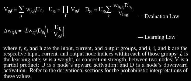
The Equations:
The Furf-I evaluation and learning laws can be summarized as follows:
The Task:
The primary empirical studies of the Furf-I algorithm used a hand-printed character recognition task. The data for this task consisted of about 9,000 hand-printed, lower-case letters and apostrophes from a single writer, rendered with anti-aliasing into two-bit deep, 12x12 images. No separation of training and testing data was made, but since the majority of the learning often happened within the first epoch, it was not a pressing issue (as pattern evaluation, which provided performance statistics, always preceded pattern training). The corpus was derived from written English text, and was presented in order, including the separating spaces (which brought the actual epoch size to nearly 12,000).
Context-Free Recognition:
The basic topology used for this task was a four-layer network, beginning with a 12x12(x4) input layer (144 four-node groups), through a 3x3(x18) middle layer, to a 28-node output group, and finally to the single-node top group. Thus, each pixel of the 12x12 input image was represented by a group of four nodes, the pixel's shade (one of four values) determining which of the four nodes would have its upward activation set to 1 while the other three nodes' activations were set to 0. The nine middle groups were connected downward to non-overlapping, contiguous, 4x4(x4) regions of the input layer, and the 1(x28) output group was fully connected downward to the middle layer and upward to the 1(x1) top group. All connection weights (the free parameters) were initialized to random values subject to the normalization constraints of the algorithm. The learning rate, L, was typically set between .01 and .05.
During unsupervised training, after each input image was presented to the input layer, the upward and downward activations were computed and the learning law applied. The output node with the highest downward activation was considered the "winner" of each trial. A matrix histogram of winner vs. actual letter identity was maintained and used to assign optimal labels to the output nodes for final accuracy assessment.
During supervised training, the output nodes were pre-labeled and their downward activations forced to represent the identity of the presented letter (one node's downward activation was forced to 1, while the rest were forced to 0). Since the downward activations were also needed for accuracy statistics, the network was run twice on each pattern--once to asses the network's guess, and once to supervise and train.
Unsupervised training produced a classification accuracy of 87%--in some trials reaching 65% before the end of the first epoch. Supervised training reached nearly 94% within the first epoch, eventually leveling out at 96%. Human performance on this data set was approximately 95% (this relatively informal measurement used one untrained subject, who had not studied this particular corpus beforehand).
Learning Context:
To study contextual learning, the previous topology was enhanced with two time-delayed copies of the output group, and a new fourth layer of 60 nodes between the now 3(x28) output layer and the top group:
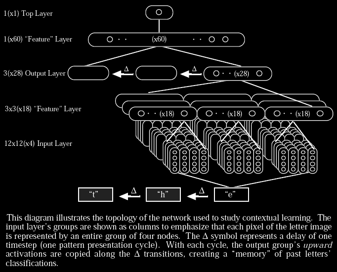
All training of this network was unsupervised. Training with the delays disabled produced the expected 87% (identical to the results obtained by the simpler architecture). Enabling the delays increased the final accuracy to over 91%. After training, disabling the delays decreased accuracy by only a couple tenths of a percent--producing a final single-letter recognition accuracy of nearly 91%. This represents a 30% reduction in error over the simpler architecture--despite the fact that, with delays disabled, the two networks are essentially identical. It appears that the upper feature layer was able to learn bi- and tri-gram statistics, and to use this information to self-supervise the lower layers of the network. [2008-06-29: Emphasis added. Fusion-Reflection in action. This is the most important point in the paper.]
Pruning:
The nature of the learning law is that unused connections tend to go to zero. After training, the network was pruned by removing any node-to-node connections with probabilities near or at zero. Approximately half of the connections were eliminated, with no notable impact on performance.
Pattern Completion:
To test pattern completion, the code was modified to accept a textual representation of the image, so that various types of noise could be added by hand. Also, the input image size was increased for better visibility. No changes were made to the algorithm itself, since pattern completion is a natural consequence of the evaluation law. The Furf network reconstructed a set of degraded patterns remarkably well (although, the test patterns were taken from among the training set). The following is a typical example of reconstruction; the question marks represent ambiguous inputs:
                              ###                       ###
                     ??????????????                    #####
                     ?       ## .#.                    ## .#.
                     ?+#+ ##      ##              +#+ ##     ##
                     ??## ##      ##               ## ##     ##
                       ???????? #                  ## #       #
                        +#+# ? #                   +#+#       #
                        +### ?????                 +###       #
                        +###       #?              +###       #
                    ?????????? #?                  ###        #
                        +##. ? #?                  +##.       #
                        +##    ? #?                +##        #
                        +##    ? .#?               +##       .#
                        +#????? ##?                +#        ##
                        +#?       ##?              +#        ##
                        +#?????????                +##
                        +#                         +#
                        +#                         +#
                        .#                         .#
Conclusion
Approaching learning from the perspective of knowledge acquisition has many advantages. In particular, by eliminating the notion of output we avoid a number of associated difficulties. Most simply, the problem of assigning meaning to the output is circumvented altogether. Similarly, there is no need to supply examples of desired output, or to supervise the learning process in any other manner. Learning laws which focus on output often neglect needs beyond that focus--such as the prerequisite knowledge required in supervised learning, or the global coordination lacking in most unsupervised algorithms. A knowledge-acquiring system, on the other hand, has guidance from beginning to end--from the simple absorption of fundamental relationships, to the global coordination of the process of abstraction.
Modeling efficacy is a simple, objective measure of a system's knowledge. Conceptually, it allows us to view and design the system as a pattern generator, which is considerably easier than trying to directly visualize the process of abstraction. Mathematically, it provides a concrete goal for gradient ascent.
Furf-I is an implementation of these principles. The empirical studies demonstrate rapid, unsupervised learning of real-world data, and give evidence of self-supervised, globally-coordinated abstraction. For a first attempt at implementing these principles, the empirical results are very encouraging.
Future Work
Expanding the Architecture
The current Furf-I architecture is severely constrained in that a node may only receive downward connections from a single group. The consequence of this is that when multiple independent features are present in the same input region, each possible combination of those features must be uniquely represented in the target group. This combinatorial explosion of features can be avoided if each node can be controlled from above by multiple groups. Techniques for implementing this re-convergence are presently being explored.
By introducing downward convergence to the topology, a number of possibilities would arise. For instance, connections could span multiple layers--allowing, at the extreme, fully interconnected networks. Recurrent topologies would also benefit from downward convergence, as discussed in the following section.
Temporal Data
The general learning principles that apply to static input apply equally well to temporal (time- varying) input. Creating a temporal model requires the same steps outlined in this paper: devise a model architecture capable of generating temporal patterns, then derive the gradient of the probability that that model would have generated the training set.
The crucial step here lies in devising the original architecture. For example, consider a Furf-I network consisting of two groups, A and B. Define B as the input/output group, and connect it upward to A. Then connect A recurrently to itself. This configuration is analogous to a node- labeled Hidden Markov Model. Pattern generation using this topology would proceed as follows: at each time step, based on the currently selected node in A, a node would be selected in B and a new node would be selected in A (due to the recurrent connection). This process can be repeated indefinitely--with the time-varying state of B defining the temporal output of the model.
With a little thought, however, it is apparent that as a generator this model is very limited: at any point in time, only a single node (within A) reflects the past state of the model. This means that if we wish to represent more than one temporal process occurring simultaneously, we must enumerate in A all possible state combinations of those processes (consider, for example, the pitch, volume, and timbre of speech, which occur simultaneously and yet are not directly correspondent with each other). This results in a combinatorial explosion in the size of the model, and hence in the number of free parameters which must somehow be determined. If it is difficult or impossible for a model to generate a pattern, it will be difficult or impossible for the model to learn that pattern. Thus the solution lies not in finding a better learning algorithm, but first in finding a better architecture.
By adding downward convergence (as described above in Expanding the Architecture) to recurrent topologies, we open the door to arbitrary connectivity. As a pattern generator, such a network could maintain multiple interacting temporal processes.
[<< | Prev | Index | Next | >>]