Sunday, June 07, 2015
Self-Supervised Learning in Bayesian Trees (and Maybe DAGs)
Another long-winded, mathy reseach log entry. Most will be happier to skip this.
See Cheap, Deep Learning with Fusion-Reflection for motivations.
Open to input, questions, comments. If anyone spots a flaw in my math, please let me know. Especially if you know how to fix it. :)
Consider the following Bayesian tree, with variables `A...D` ultimately causing some pattern `X` (here composed of three separate parts):
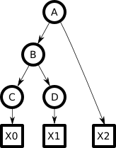
Here `A...D` are discrete state variables, each taking on one of some fixed number (`N_A...N_D`) of states or values. Each `X` is some observable, such as a patch of a photographic image. Assume we know the direct mappings between the variables and each `X` so we needn't concern ourselves with the details of `X`. In particular, assume we can generate an `X0` from any `C_j` and so on, and likewise can compute `"P"(X0|C_j)`--the probability of a generating a given `X0` from a given state (`j`) of `C`. Each arrow in the graph is associated with a weight matrix specifying how each state in the parent influences each state in the child. So the arrow from `A->B` implies an `N_A xx N_B` weight matrix, whose elements I will call `P(B_i|A_h)`. The single-state "root node" (parent of `A`) is not shown here, but implies a `1 xx N_A` weight matrix defining `"P"(A_h)`. This tree is binary (two children per node) but the math all generalizes to N-ary.
The node `B` here is representative of any node in the middle of any Bayesian tree, so we can analyze that and assume it will generalize (see Appendix for details):
| ` "P"(X0|B_i) = sum_j P(C_j|B_i)"P"(X0|C_j)` | (1) |
| ` "P"(X01|B_i) = "P"(X0|B_i)"P"(X1|B_i)` | (2) |
| ` "P"(B_i|X) = "P"(X01|B_i) sum_h (P(B_i|A_h)"P"(A_h|X))/("P"(X01|A_h))` | (3) |
Equation (3) is the posterior state of `B` given all the evidence, which is usually the thing we care about.
Equations (1) and (2) are problematic in a deep network because they rapidly exceed the floating point range (the sum in eqn (1) prevents us from simply using log values). However, note that scaling any `"P"(X|V)` by a constant in equations (1) or (2) will cancel out in equation (3), so we can, say, simply normalize them to keep them in a good range. Doing so prevents us from using automatic differentiation, since those scaling factors are what propagate those otherwise local gradients all the way to the root of the tree, but we can still compute the gradient symbolically. (Technically, we could maintain a parallel sum of log scaling values, and add those in at the end, which would make the auto-diff work again, but we really don't need auto-diff here -- see below.)
Equation (3) can also be written this way (by expanding the denominator with eqn (1)):
| ` "P"(B_i|X) = sum_h "P"(A_h|X) (P(B_i|A_h)"P"(X01|B_i))/(sum_n P(B_n|A_h)"P"(X01|B_n))` | (4) |
In this form it is evident that if we wish to sample a posterior state of the whole network, we can begin by sampling from `"P"(A_h|X)`, resulting in some single `A_h` being selected, and then:
| ` "P"(B_i|A_h, X) prop P(B_i|A_h)"P"(X01|B_i)` | (5) |
From which we can (normalize over `i` and) sample to select some `B_i` and so on down the tree.
To make this more concrete, let's ditch the probabilistic notation for a moment in favor of vectors and matrices as we might implement this in a program. In particular, let's call equation (2) the upward value of `B`, designated by `hat B`. This is an `N_B`-sized vector (over `i`), which we can normalize if we wish (since any constant scaling washes out in the end). Likewise, let's call a sample drawn from equation (4) the downward value of `B`, designated by `bar B`, which represents a posterior sample from the network given all the evidence, and is a one-hot vector the same size as `hat B`. Call `W_(BC)` the matrix of `P(C_j|B_i)` for all `i, j`. Then, for any number of children `C` (i.e., here `C` represents `C, D, ...` in the figure):
| ` hat B prop prod_C W_(BC) hat C` | (6) |
| ` bar B ∼ bar A W_(AB) o. hat B` | (7) |
Or in code (where 'dot' includes matrix-vector products):
B_up = normalize(dot(Wbc, C_up) * dot(Wbd, D_up) * ...)
B_dn = multinomial_sample_onehot(normalize(dot(A_dn, Wab) * B_up))
Or, if V_dn is stored instead as an integer index:
B_dn = multinomial_sample_int(normalize(Wab[A_dn] * B_up))
Note we could also use (3) directly without sampling to get the full posterior distribution for each variable. I give the sampling example here because I find it interesting how simple equation (5) is, and because it side-steps some issues in DAGs...
Moving on to DAGs...
Consider the following Bayesian network, with variables `A...D` ultimately causing some pattern `X`:
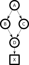
The downward convergence creates a new case we need to handle in our generative model which, for various reasons, we'll choose to do as a normalized element-wise product of each parent's implications (essentially mirroring equation (2)):
| ` "P"(D_k|B_i,C_j) -= (P(D_k|B_i) P(D_k|C_j))/(sum_m P(D_m|B_i) P(D_m|C_j))` | (8) |
Note here `"P"` refer to true probabilities (from normalized distributions), while `P`, our stored model parameters, are merely factors of eventual probabilities. I'm retaining the (softer) `P` notation as a conceptual reminder of their role in the graph.
Most of the tree math stops working here, unfortunately, chiefly because `B` and `C` are no longer independent with respect to `X`. To illustrate by example, consider the following model:
| ` N_B = N_C = 2 ; N_A = N_D = 4` | (9) |
| ` {:(P(D|B_0),= [1,1,0,0]), (P(D|B_1),= [0,0,1,1]), (P(D|C_0),= [1,0,1,0]), (P(D|C_1),= [0,1,0,1]):}` | (10) |
This, in effect, is a multiplexor which takes the 2-bit binary value represented by `B, C` and selects one of four corresponding states in `D`. So:
| ` {: (B_0 C_0,-> D_0), (B_0 C_1,-> D_1), (B_1 C_0,-> D_2), (B_1 C_1,-> D_3) :}` | (11) |
For now let's have `A` mirror `D`, so that:
| ` P(B_0|A) = P(D|B_0)` | (12) |
And so on. (In other words, `A` is de-multiplexed into binary `B, C` and then multiplexed back out to `D` so that `D = A`.)
Let's say we observe:
| ` P(X|D) = [0,0,1,0]` | (13) |
In other words, only `D_2` can generate `X`. From this the model can easily infer:
| ` X -> D_2 -> B_1 C_0 -> A_2` | (14) |
Seems fine. But what if:
| ` P(X|D) = [0,1,1,0]` | (15) |
That is, both `D_1` and `D_2` can equally well generate `X`. Now our valid middle layer states are either `B_0 C_1` or `B_1 C_0`, but not `B_0 C_0` or `B_1 C_1`. This means there is no way to encode `B`'s and `C`'s distributions separately (i.e., in a way that assumes they are independent). The usual solve here is to join variables into cliques* or whatnot, but that's not practical here where I am aiming for very wide layers.
My first thought, and what I have been testing empirically with some success, is to just use the tree math, with downward sampling, noting that equation (5) becomes this:
| ` "P"(D_k|B_i, C_j, X) prop P(D_k|B_i)P(D_k|C_j)"P"(X|D_k)` | (16) |
This is prone to be wrong (optimistic about possible combinations) on the way up, but is then forced to construct a self-consistent picture on the way down (since sampling only selects one state for each variable, it can't fake a good pattern with spurious combinations). Right now I am using the tree code unmodified, but I should probably be doing some form of rejection sampling in order to properly discard the spurious combinations that do make it through the upward pass.
I briefly considered sampling on the upward pass, but my sense is the ambiguity can be pretty high at that stage, and with many parallel variables (wide layers) the combinatorial explosion would effect a very inefficient search.
Conversely, using the optimistic approach on the upward pass is likely in practice to result in a correct answer despite transient optimism along the way. I say "transient" because the spurious combinations that are implied by one layer are likely to be discounted by the next as more context is brought in. For example, consider an OCR model of printed words. A given letter may be italic or regular, and some visual symbols like "/" could be seen as a regular slash or an italic I. The "optimism" of the (bad-math) upward pass would also consider, upon seeing the "/", a regular "l" and an italic "/". But rather than compounding, these sorts of errors are likely to wash out--because the next level up will be looking at whole words, and will simply dismiss (due to multiplicatively combined probabilities) the possibility of an italic letter in the middle of a regular word, or a slash where only an "l" makes sense.
Put another way, with many variables each having a few possible states (given the input), finding the coherent combination through sampling could take forever, but conversely the more variables there are, the more likely the spurious possibilities from the optimistic approach will average out, leaving the true pattern (and posteriors) as the dominant signal.
Hand wave, hand wave. At this point I don't know the best way to estimate or sample the posterior states, but faking it with the tree code is doing alright so far. I have added the (soft) constraint that the denominator in equation (8) should be approximately 1, as I suspect this eliminates some of the source of error of the tree approximation, but I don't have a solid justification for this. (Could be a spurious combination created by my faulty brain...)
Oh, which reminds me: Q: What do you call it when an input induces coordinated spurious combinations that don't wash out? A: Optical illusions? Just a thought...
Moving on...
We can compute the posterior state in the tree, and to some degree approximate a sample from it in the DAG. So how do we train it?
As implied a couple entries ago, we can use the principles of the EM algorithm to break the problem in two: First, find the posterior state of the network given each pattern in our training set from our current weights (Expectation)--which we addressed above--then adjust the weights to fit that expectation (Maximization); repeat. Handwavingly, I'm going to claim you can do the same thing on mini-batches by following the gradient toward the EM convergence point. One might call this Stochastic Expectation-Maximization (which may or may not already exist; I don't have time to fall down another Google rabbit hole so I'm not going to check).
The tricky bit is the convergence from `B` and `C` to `D`, so we'll focus on that.
Recall we've declared the generative model to work like this:
| ` "P"(D_k|B_i,C_j) -= (P(D_k|B_i) P(D_k|C_j))/(sum_m P(D_m|B_i) P(D_m|C_j))` | (17) |
This is an example of equations (1) and (7) from Gradient of Auto-Normalized Probability Distributions, with:
| ` {: (F_k,-= P(D_k|B_i) P(D_k|C_j)), (bar "P"(bar D_k),-= "P"(D_k|B_i, C_j, X)) :}` | (18) |
Which provides:
| ` {:(del_(P(D_k|B_i)) log "P"(bar D_k|B_i,C_j),= (del_(P(D_k|B_i)) P(D_k|B_i))/(P(D_k|B_i)) ["P"(D_k|B_i,C_j,X) - "P"(D_k|B_i,C_j)]), (,= 1/(P(D_k|B_i)) ["P"(D_k|B_i,C_j,X) - "P"(D_k|B_i,C_j)]):}` | (19) |
Recall `P(D_k|B_i)` is just our stored, scalar weight. We can clean up the above by choosing instead to store log weights, so that we get:
| ` {:(del_(log P(D_k|B_i)) log "P"(bar D_k|B_i,C_j),= (del_(log P(D_k|B_i)) P(D_k|B_i))/(P(D_k|B_i)) ["P"(D_k|B_i,C_j,X) - "P"(D_k|B_i,C_j)]), (,= "P"(D_k|B_i,C_j,X) - "P"(D_k|B_i,C_j)):}` | (20) |
It doesn't get much simpler than that! Stated plainly: if our generative model (for child variable `D`) is to multiply the distributions implied by each parent variable's state (`B_i` and `C_j` for some known and particular `i` and `j`) and then re-normalize (to get `"P"(D_k|B_i,C_j)` for all `k`, aka `"P"(D|B_j,C_j)`), then the gradient to optimize the (log) components of those distributions (our "weight vectors" `log P(D|B_i)` and `log P(D|C_j)`) is simply the linear difference between the witnessed (here: posterior) distribution of `D` (aka `"P"(D|B_i,C_j,X)`) and our generated/expected distribution of `D` (aka `"P"(D|B_i,C_j)`). Note that this is all conditioned on having selected `B_i` and `C_j` from the posterior distribution in the first place--so this method assumes we have sampled those during the downward pass.
The python numpy* code to train one pattern might look like this:
def one_hot(V, i):
    "Returns a probability vector for the states of V representing certainty that V is in state i."
    a = np.zeros(V.n)   # V.n is number of states in variable V
    a[i] = 1.
    return a

def train1(B, C, D, i, j, k, lrate):
    """This says we have observed parent variables B, C, and child D, in (integer) states i, j, and k,
    and we wish to increase the likelihood that B,C=i,j will generate D=k in the future.
    Lrate is the (scalar) learning rate.
    """
    predicted_D   = np.exp(B.weights[i]+C.weights[j])     # V.weights is a matrix with shape (num_parent_states, num_child_states)
    predicted_D  /= np.sum(predicted_D)                   # Normalize into a proper probability distribution. (OPTIONAL: See text.)
    actual_D      = one_hot(D, k)                         # We could also accept an observed softer distribution, but this works if D has definite state.

    err           = actual_D - predicted_D

    B.weights[i] += lrate * err
    C.weights[j] += lrate * err
So, super simple, and note that the components of err are bounded from -1 to 1 so it is also very well behaved. In practice, the code is even simpler than this because both predicted_D and actual_D are likely to have already been computed by the evaluation passes.
Also, note that it is the same gradient for both parents (or, more generally, as many parents as there may be). What causes them to diverge is not different gradients (err) on a given example, but rather that the i's and j's correlate differently with the k's over time. That is slightly more evident in this alternate implementation, for when we have observed distributions rather than explicit states:
def train2(B, C, D, PB, PC, PD, lrate):
    """This says we have observed parent variables B, C, and child D,
    in (independent) state distributions PB, PC, and PD respectively,
    and we wish to increase the likelihood that those B,C combinations
    will generate D in the distribution PD in the future.
    Note this is (almost) equivalent to repeatedly sampling B, C, D from PB, PC, PD
    and calling train1() above.  (See text for caveats!)
    """
    predicted_D  = np.exp(PB.dot(B.weights)+PC.dot(C.weights))  # Note if PB is one_hot(B, i) then PB.dot(B.weights) = B.weights[i]
    predicted_D /= np.sum(predicted_D)                          # Normalize into a proper probability distribution.
    actual_D     = PD                                           # Actual D distribution directly provided.

    err          = actual_D - predicted_D

    B.weights   += lrate * np.outer(PB, err)                    # Err is added to B.weights[i] in proportion to PB[i]
    C.weights   += lrate * np.outer(PC, err)
There is a caveat here, however: If some B[i], C[j] combinations result in very different normalization factors for predicted_D, then train2 is not really equivalent to sampled calling of train1.
This normalization variability is the issue I tried to address previously by adding a cost term of [sum(predicted_D)-1]**2, which forces the converging distributions to be naturally normalized. That worked (in an automated differentiation setting) but makes for a poorly behaved gradient (steep canyon walls). Hand-wavingly, note if you simply drop the normalization step of predicted_D, you get the same effect. (Harder to justify for train2 than train1.) That is, delete one line of code from train1 and it now also trains predicted_D to naturally sum to 1. (Tip: If you divide by the number of states instead of normalizing, then initial log-weights of 0. will be in constraint, and more generally the weights will tend to hover near zero which can be handy. Since we are sampling on the downward pass here, the initial weights can literally all be zero and you will still get divergence thanks to the randomness introduced by the sampling.) It's not immediately clear how this constraint and the optimization objective might balance against each other, but empirically so far it does tend to keep sum(predicted_D) fairly close to 1 (or the number of states) as intended, and the network trains much faster than with the constraint/auto-diff method, with similar end-results.
Hopefully the code snippet example makes the math a little more concrete.
I added a couple of new case patterns to the seven-letter word corpus I mentioned a couple entries ago (and consequently am stripping case from the generated patterns to make them easier to read...).
Here's from a network with two hidden layers of ten 20-state nodes each:
atleoto glaseny vurirer aritoon egcrute corstwr fotturn puoiost beslews tanates sannews aulteps sweurer asrtras danveys scolers timoles slalful cluttes gwakker ceclens vedaacs reteond sunaice auarder teaauts delents didlers bubrens nemrake wragned seerons rimpsed perenin veaslle ordeits lrclide soosacs scriver hirtiar spiller aerfher tebulea rirkled dissieg basters renress aersiss gexvinh enjouns
Same but with a hack that encourages all states to be used. Turned out one state was tending to learn the prior distribution of the children and would dominate so quickly that all the other states got pushed to near zero likelihood before they got a chance to compete. Not sure if this is any better:
couuces dente's aunalrs enstled laggary coofand bradins mevises ansuied brapper puoring lalimer icpapel irdsled fanslrp pigarew cuakout vinelin glabirg tradnin sphaier lomgagd inasele batesow sronerd slogone soxtted enhosts siohons intrine sprrohy procker cortets doising lanaile jutwley ambrawr honktrs pepacis toerect devorve camoees buptier sptties jametts corec's petetes croiney cablres fendrea
The most promising result is that under some conditions it does learn to factor out the capitalization rules (currently five distinct rules) from the letter sequence. That is, one set of parent variables dictate the word, and another parent variable dictates how that word should be capitalized. It was able to learn this despite the alphabet coming in as an unlabeled set of 53 tokens. So, simply by seeing the same words appear with different capitalizations, it is eventually able to associate "a" with "A" (amongst the parent variables that specify the word) and "A" with "B" (amongst the parent variable that specifies the capitalization rule). In other words, it does appear to be usefully factoring the pattern space. However, it's not doing it as quickly or consistenly as I would hope, so there is more work to do. (Rejection sampling, etc.?)
Thanks to Colin Green* for useful discussions.
Appendix: Derivation of Downward (Posterior) Evaluation Law in Trees
The limitations imposed by the topology give:
| ` "P"(X|B_i) = "P"(X01|B_i)"P"(X2|B_i) -> "P"(B_i|X) = ("P"(X01|B_i)"P"(B_i|X2)"P"(X2))/("P"(X))` | (21) |
| ` "P"(X|A_h) = "P"(X01|A_h)P(X2|A_h) -> "P"(A_h|X2) = ("P"(A_h|X)"P"(X))/("P"(X01|A_h)"P"(X2))` | (22) |
| ` "P"(B_i|X2) = sum_h "P"(A_h|X2)P(B_i|A_h)` | (23) |
Substituting (22) into (23) into (21) gives:
| ` "P"(B_i|X) = "P"(X01|B_i) sum_h (P(B_i|A_h)"P"(A_h|X))/("P"(X01|A_h))` | (24) |