Friday, May 22, 2015
Cheap, Deep Learning with Fusion-Reflection
Wherein I extol the virtues of self-supervised learning via generative models (AI geekery).
Training a function to compute labels for images is a typical case of supervised learning. We present a large corpus of rich inputs (such as images) along with human-provided targets (usually much simpler, such as one or more of N discrete labels), and then follow the gradient (over the free parameters of the function) of the function's output vs. the desired targets. Often that "function" is in the form of a "neural network", typically a layered collection of individually-simple computational units with multiplicative input weights as their free parameters.
The trouble in the past with this was that a network with enough layers to compute something as challenging as general image labeling would have an initially diminutive gradient, due to the random mixing effect from each layer to the next in a randomly initialized network, and so they were very hard to train. We got past that mostly by... throwing more hardware at it, and using slightly better gradient following algorithms. And thus Deep Learning was born by Caesarean section. (Convolutional networks, for those thinking it, are nothing remotely new, although they are key to this working at all as explained below.)
The trouble remains, however, that the training information is not only limited to the very small number of bits we humans are patient enough to provide, but to the very small number of bits in the simple output targets period. Consider especially when a naive network is just getting its start in the world, knowing nothing yet about images at all. We show it a million colored dots and say this is a dog. We show it another million colored dots and say this is a car. As far as the network is concerned at this point, this is all just random snow. Furthermore, unless the training set is very restricted (say cropped and scaled to mostly just contain the object of interest) there's very unlikely to be any measurable correlation between any dot's color and the image label. This means we're relying on there being some path through the layers which, by chance at the start, at least slightly embodies a relevant generalization--some more abstract pattern which does exhibit a measurable correlation, however slight. Convolutional networks effectively cheat here, by hard-coding a broad class of such generalizations right into the network architecture. I'm not against cheating, but it begs the question: does it have to be this hard in the first place? The answer is: Nope.
The reason it's hard is because it's a terrible setup: Imagine we're workers inside the neural network, doing our computations and passing the results on to other workers and so on. At the image end of the network, we're gathering up pixels, mushing them together randomly, throwing this garbage at the next layer, which then mashes it up further and so on, until finally someone at the far end gets this pile of garbage and is told "that's a dog". Bear in mind, they're looking at a pile of random garbage at this point. This is already bad enough, but then they basically mix up the garbage and send it back, with notes that say more garbage here, less garbage there, and eventually this gets back to you in the form of a vague hint that's probably wrong but over a million examples might, just might, average to a useful trend. Critically, the only hints you are allowed to act on are these cryptic notes coming back to you from a round trip through the telephone game with the guy on the far end of the garbage heap. That is, you're not allowed to, say, just look at whatever patch of the image is yours and start taking notes on what you see.
I go through that long-winded description to drive home that crucial point--the input layer of the network is looking right at the image, but is only allowed to learn whatever happens to correlate with the faint and scrambled remnants of some low-bit training signal from far far away. Kind of a waste, no? I mean... it's looking right at the image!
There's a lot of information that can be learned about images (that will ultimately help us classify them) right from the images themselves, without even considering those far-away labels. We can worry about the labels once we have a better general understanding of images... So how do we do that?
This is where modeling efficacy comes in. Rather than tasking our network with mapping images to labels, we task it with modeling images. That is, we just point at the images and say: I want you to be able to do that. In effect, we're asking it to learn to paint instead of label. At first this seems like a much much harder problem. In some ways it is, but it also a much more immediate problem in that your source and target examples are one in the same--which means there are only as many layers of abstraction between them as your own understanding introduces.
To clarify that last point, consider that you can make some headway in modeling images just by observing the distribution of raw pixel values. Maybe they form a normal distribution, or whatever. With nothing more than that very simple thing you've actually made huge headway in making images that are very measurably more like real images. Then maybe you notice neighboring pixels are correlated. Model that, and you've made more measurable headway. Then you notice that non-correlated pixels often line up. Poof, you've discovered edges. Now you're modeling images even better! And so on and so forth.
But how do we "measure" something so abstract as how well we are modeling images? One way, which I'll stick to here, is to ask the question: If you painted a bunch of random images from your current model, what are the odds they would be exactly the images in the training set? This of course would be a tiny, tiny number, because it's the product of very many small probabilities. In the simplest case where we are only modeling individual pixel distributions, it is the product over the probabilities of generating each pixel of each image. But that's fine--it turns out what makes it so small is also what makes it a fantastic gradient to follow.
Take its negative log so we turn that product into sums, and this reveals a very nice property: this "cost function" (the negative log probability of our model generating our training set) is, in most practical cases, a sum over the costs of smaller components (such as individual pixels, or more typically a hierarchy of features), and over all our examples. Because the gradient (slope) of a sum is just the sum of the gradients of its parts, this means as long as there is an easy improvement to make anywhere, on any example, in any way, we have a measurable, usable gradient. In other words, we don't have to make any connection to dogs vs. cars whatsoever, we can simply notice that edges are common in images and we've made measurable progress. Or, more to the point, we can see that we can make measurable progress by learning that there are edges, and so we do. The fact that we're nowhere near telling dogs from cars yet doesn't slow us down in the least.
By contrast, the only way to learn about edges in a (purely) supervised network is through a very indirect route in which noticing edges ultimately helps us distinguish dogs from cars. This is nearly impossible at the start, and gets better almost incidentally as we learn generalities of images and how they correlate with our labels, but this (edge) gradient is never as strong in the supervised case as it is right from the start in the modeling case.
I started this entry a couple of days ago, and then coincidentally Andrej Karpathy posted this yesterday which is rapidly making the rounds:
The Unreasonable Effectiveness of Recurrent Neural Networks
He attributes the cool factor to the temporal aspect of RNNs. I agree with everything he says about the goodness of the temporal approach, but I don't think it's actually the key to what's making his examples so compelling. If you look at what he's done, you'll note it is exactly an example of what I describe above. His generative model happens to proceed from left to right, but it is a generative model: You can start it from scratch, push a button, and it spits out a random, generated example. The cost function he is using is the cross-entropy of each next letter his model generates vs the training sequence, implicitly summed over all the letters in the sequence and all the sequences in his training set. Jointly, this is precisely the log probability of his model generating his training set. Poof.
He and others have also used RNNs to do things like map from images to labels, which is sort of a hybrid of modeling and supervision. I would expect/predict that the sticky points of those experiments have had to do with working around the inherent limitations of the supervised aspect as explained above, and that they could be greatly improved by finding ways to turn them into pure modeling problems first, with the supervised task added on only at the periphery.
But this raises the question of how to implement and train a generative model of images. I agree with Andrej that attentional, temporal methods are ultimately vital here, but it's my sense that the momentary model directed by that attention needs to operate roughly in a parallel, spacial manner similar to current (convolutional, etc) approaches. So let's look at those.
One of the more straightforward and well studied ways to build a generative model is with Bayesian networks. People tend to associate those with more symbolic approaches, or at least expert systems with hand-labeled, high-level concepts and whatnot, but the principles of Bayesian networks apply just as well to unlabeled, hierarchical deep networks just like any other neural net. In fact, winner-take-all type arrangements of (real) neurons, where you have N excitatory neurons grouped by a common inhibitory neuron, can be viewed as a single discrete, N-state Bayesian variable.
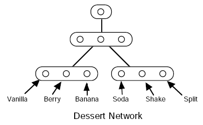
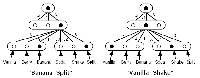
To generate a pattern from a hierarchical Bayesian model with top-down causality, you can start with the root node at the top (a 1-state variable, always True), compute the probabilities for its children (the layer below), randomly select their states accordingly, and then continue to their children in the next layer down, and so on until you reach the bottom--which would be the pattern (input/output) layer.
See Furf I (scroll down to Furf Nets) for an example of this with tree-structured Bayesian nets. The evaluation and learning laws are covered there as well, but in short: You simply compute the probability of generating the training set, and follow the gradient. For the tree structured case that probability computation proves trivial, and with modern automatic differentiation the gradient comes along for free. (I tested this recently--yep, it works.)
In the Furf paper, I derived the gradient by hand. One advantage of that was to see how exactly the learning works. I've been speaking abstractly about gradients of total log generative probabilities and whatnot, but what does this actually end up looking like as a learning law? Turns out, one way or another, the learning law ends up relying primarily on the posterior distribution of states given the input. That is, we present an input (such as an image) and ask: Presuming we had just generated this input (image) from the network, what are the odds we had selected any particular state in each variable along the way down? In the case that one of those variables is, say, the identity of a letter we are rendering into an image, answering this question is akin to asking "What are the odds this image is the letter A? What are the odds this image is the letter B?" and so on. (In other words, it happens to be exactly what you would want out of a supervised network. And you can often get this for free without ever having to supervise. But I'll get back to that.) Once you have that posterior distribution for each variable, the learning law essentially proceeds by simply keeping track of what percentage of the time each child state is true for each parent state and... that's the model. In other words, it just comes down to counting. It's that trivial. Well, almost: Because the posterior states are predicted in a distribution, we have to do a soft version of same, wherein we weight the count by the probability of the parent. In effect, the parent node's "activation" defines the plasticity of its downward connections, which are adjusted in the direction of each child's distribution. Note that this is essentially Hebbian learning. In batch mode, it is the EM algorithm. (Interesting the two are equivalent, eh?)
But how do we get the posterior distribution over variable states given an input? In the tree structured case this is fairly easy, but it requires two passes: One from the bottom up, which computes the probability of the portion of the input visible from each variable given each state of that variable, and then one from the top back down, which computes the probability of each state of each variable given the entire input. In other words, the information is progressively fused into more abstract and global information on the way up, and then reflected back down in a way that makes each variable aware of the entire context.
This in itself is a very interesting and useful behavior. Consider the case of a handwriting recognition system that sees images of characters in the context of words. Looking at a particular letter locally and out of context, you may be unsure whether it's an "i" or an "l" for instance. During the upward pass, this ambiguity is exactly what we see, because the upward pass computes the context-insensitive distributions. That is, both the "i" and "l" states for the variable encoding that letter's identity will be given some weight, while the others will mostly be near zero. But let's say the next level up in the network is a variable that overlooks many characters at a time and recognizes whole words. The following letters appear to be a couple of "o" or "0"s and then a "k". Of all the known words, only "look" matches, and so even during the upward pass, this fusion of ambiguous information results in a very non-ambiguous word recognition. This is immediately useful if you want to know the identity of the word (and note that it was found quickly--in one bottom-up sweep). But note what happens now with the downward pass: The word-level variable now reflects that fused information back down to its children, and informs the first letter that it is in fact an "l" not an "i", and the second letter that it is an "o" not a "0" and so on. As noted above, these posterior states are used for the learning. This means...
The network is self-supervising. The training "label" here was generated by the higher levels of the network itself. But how did it get there in the first place, you might ask? Prior experience. To be clear, the network never knows that one state is "l" and another "i", it just knows they are states 7 and 2 or whatever. But the word level learns over time that 7-5-5-9 ("look") is a common sequence (more common than the alternative interpretations because, on average, the l looks more like an l than an i, the o's look more like o's than 0's, and so on), and this in turn biases the posterior interpretations of the letter images in context to be treated more like 7-5-5-9 ("look") than 2-3-3-9 ("i00k"). What makes state 7 here an "l" is not a label (the network still doesn't know it's associated with the human label "l"), but that it also shows up in lots of other words (all the other words with "l"). I.e., it is a combination of co-participation in other words, and multiple examples of the same words, which encourages a natural partitioning of classes. And these classes in turn become self-supervised training targets provided by each layer to its children below.
However, note that this top-down information is strictly contextual refinement. Without it, the posterior distributions aren't lost, they are simply not improved by context. That is, no matter how many layers there are above us, it doesn't take away what we can observe (and hence learn) in the strictly bottom-up mode. A sub-network that just sees one image letter at a time can still learn to model letters. It just won't learn as well as it would eventually provided top-down context. This is the key advantage over a supervised network: We rely first on local information, and later refine with information from further and further away; whereas a supervised network in a sense is forced to do the opposite--look for a thread of happenstance correlation from one end all the way to the other, and then amplify that thread until it provides enough information (a strong enough gradient pushing through many layers) to start meaningfully training locally.
The tree structured case is easy to understand and the math is pretty, but it lacks the ability to "factor" our pattern space into separable components. Say, for instance, we are doing OCR and there are various fonts and styles (bold, italic, regular). We would like the font, style, and letter identities to be separate variables which converge downward into a particular generated letter image. That is, we would like a DAG* rather than a tree.
Suddenly the math stops being pretty. Perfect inference in such a DAG is, I believe, NP complete, in that you have to effectively enumerate over all combinations of states. There's a huge body of literature on related approximate methods, etc.. However, we can simplify the problem somewhat by restricting how the downward probabilities converge. In particular, setting the child distribution as a normalized, element-wise product of distributions provided by each parent seems a natural choice, as this mirrors the analogous computation that is done during the upward pass. Unfortunately, the fact that the normalization constant varies with different combinations of parent states means the equations remain non-factorable. Hinton addresses this somewhat via Contrastive Divergence[pdf], but I don't believe you can stack those meaningfully (no fusion-reflection).
An approach I've been playing with recently is to simply train the normalization constant (for the downward convergence) to be 1. (This may seem like a severe constraint, but it's not as bad as it seems. More about that another time perhaps.) I'm doing this presently by just adding a strong normalization penalty to the cost function. This is a terrible thing to do to any gradient-follower because it creates steep canyons everywhere, so I don't recommend it. But it does work--it's just very slow. (I expect this can be improved with a manually computed gradient, probably using reverse inhibition in the spirit of GHA*.) For now I'm leaving the rest of the math the same as in the tree structured case. This isn't really correct, as it credits spurious combinations when the upward distributions are non-sparse, but it tends toward a correct solution as they become more sparse (which they tend to with training).
I need to run some more interesting tests, but for a quick trial I made a simple network to generate seven-letter words. There are about ten thousand words in the training set, and each of them occurs three times as all lowercase, all caps, or first letter cap (so 30k words in total).
Words generated by an untrained network look like this:
BKvlUpw GTOuMwW EVhcfta eKCbyjz VIeiekN zHnJaBl WijYOTr wAZqLNl ZovRzXV fbjOfGC QYfFnkF bDBkaNE JRqXwIr PvPNKxU uxSAGyn CuuGuYb IozpcZV iYKiKRm bKjOeYP wckNHtY DHVRvZm ryBUKNR ekwfLrl bHiRFCv xCAHnAt bAmgPhW KMWVcTU oxsqHRO rudLoIb fBqTokB rMwaFMh WemDHQw gkIZLDg pp'OsKm HOepz'F ZYUqqUx hrOFpHU PBJiwql lnsKxBG uGhzRbU SRzEkKo HhlIBrB LS'FyrF ek'MumL Y'kqtSM lEehoqO PDfOnfS hrAHLDb UCKPVUI hfKCsYI ...
A (SMORMS3) trained network with one hidden layer of a couple of 500-state variables generates words like this:
ANBENRS mesttes skenner PIPPLER lottier capioly AROOMED viocass INRGITD otnwing Stirisn GORPONS Cerrios LOSLING weavers Rmoifry lightls Miuring laspags BLAMANT blurhed GFBBFKH tipping BLESSES Molubny tiwying AEPEALS DHPARRS Hecadly remarls fankhes morsa's Mersing innuins BENROEK Renhuck Ralanzs mhaping CYVINGY Dliepel assting rettits SRDGIZW coomers qerfing Breteen Stripes harraan refibed inchaps ...
Of note, there are still some turds in there like SRDGIZW. On inspection, it turns out these are places where the downward convergence doesn't normalize. In other words, there are (detectably) "invalid" combinations of hidden layer states. Presumably this is happening because the normalization penalty is applied to the posterior state, which means hidden state combinations that never happen in the wild are never forced to normalize against each other. But because the next layer up from there is the root node, which only has one state, correlations between the hidden states can't be learned, and hence bad combinations can't be avoided.
I tried another architecture with a first hidden layer of 20 10-state variables, and a second hidden layer with 1 100-state variable. It's still generating turds. I'll need to look into why... (But this hasn't trained nearly as long as the other so perhaps it will improve.)
seszaie Mocuwls tlinnes jeasawd Hotrurt Ponottn sessing goucned Calonts MATQICA AOVUREH Seganta chumbed rextens Surdark crabped MPTLING fuivaps Becsern Morence oibsery deefens peciris mnpored NEAKING RECETES tdgnina nwtting Rmpited POUTING woiding HORFAGE ALETIRS FULZING mrssert Faskles COOIICS Panangs cukting caliers Revatel SLETHED Saggies ANDEMES Uokegel Cooxars HAILESS emltlds GPEACED STAPMSD ...
Note, however, I am intentionally picking network configurations that are not at all easy. Here we're asking it to generate 30,000 specific words with 300 "neurons"...
Anyway, more work to do on the DAG models. But hopefully some of the above provides some inspiration for considering generative models.
[Update, October 2017: see also Probability Density Mapping]