Monday, December 11, 2006
Netflix Update: Try This at Home

[Followup to this]
Ok, so here's where I tell all about how I (now we) got to be tied for third place on the netflix prize. And I don't mean a sordid tale of computing in the jungle, but rather the actual math and methods. So yes, after reading this post, you too should be able to rank in the top ten or so.
Ur... yesterday's top ten anyway.
My first disclaimer is that our last submission which tied for third place was only actually good enough for ninth place or so. It landed where it did because, just for giggles and grins, we blended results (50/50) with Jetrays who had a similar score to us at the time.
Second, my friend Vincent has been manning the runs on his desktop machines, diligently fine tuning and squeezing out every last bit of performance possible with whatever controls I could give him (not to mention learning python so he could write scripts to blend submissions and whatnot). In short, almost all my progress since my last post has been due to other people. In the meantime I've implemented a handful of failed attempts at improving the performance, plus one or two minorly successful ones which I'll get to.
Now for the method to the mathness, begining with a review of the problem:
Netflix provided 100M ratings (from 1 to 5) of 17K movies by 500K users. These essentially arrive in the form of a triplet of numbers: (User,Movie,Rating). E.g., one such entry might be (105932,14002,3). Times 100 million. Now go make sense of it. In particular, for (User,Movie,?) not in the database, tell me what the Rating would be--that is, predict how the given User would rate the given Movie.
I'm tempted to get all philosophical on my soap box here and go into ways of thinking about this stuff and modeling vs function mapping approaches, yadda yadda, but I know you all are just here for the math, so I'll save that for the next hapless hosteler who asks me what I do for a living.
For visualizing the problem, it makes sense to think of the data as a big sparsely filled matrix, with users across the top and movies down the side (or vice versa if you feel like transposing everything I say henceforth), and each cell in the matrix either contains an observed rating (1-5) for that movie (row) by that user (column), or is blank meaning you don't know. To quantify "big", sticking with the round numbers, this matrix would have about 8.5 billion entries (number of users times number of movies). Note also that this means you are only given values for one in eighty five of the cells. The rest are all blank.
Netflix has then posed a "quiz" which consists of a bunch of question marks plopped into previously blank slots, and your job is to fill in best-guess ratings in their place. They have chosen mean squared error as the measure of accuracy, which means if you guess 1.5 and the actual rating was 2, you get docked for (2-1.5)^2 points, or 0.25. (In fact they specify root mean squared error, affectionately referred to as rmse, but since they're monotonically related it's all the same and thus it will simply hurt your head less if you ignore the square root at the end.)
One additional tidbit is they also provide a date for both the ratings and the question marks, which aside from giving you more rocks to try to squeeze blood from also implies that any cell in the matrix can potentially have more than one rating in it. This would seem to violate the whole matrix analogy but as it happens that's mere foreplay compared to what follows.
Imagine for a moment that we have the whole shebang--8.5 billion ratings and a lot of weary users. Presumably there are some generalities to be found in there, something more concise and descriptive than 8.5 billion completely independent and unrelated ratings. For instance, any given movie can, to a rough degree of approximation, be described in terms of some basic attributes such as overall quality, whether it's an action movie or a comedy, what stars are in it, and so on. And every user's preferences can likewise be roughly described in terms of whether they tend to rate high or low, whether they prefer action movies or comedies, what stars they like, and so on. And if those basic assumptions are true, then a lot of the 8.5 billion ratings ought to be explainable by a lot less than 8.5 billion numbers, since, for instance, a single number specifying how much action a particular movie has may help explain why a few million action-buffs like that movie.
A fun property of machine learning is that this reasoning works in reverse too: If meaningful generalities can help you represent your data with fewer numbers, finding a way to represent your data in fewer numbers can often help you find meaningful generalities. Compression is akin to understanding and all that.
In practice this means defining a model of how the data is put together from a smaller number of parameters, and then deriving a method of automatically inferring from the data what those parameters should actually be. In today's foray, that model is called singular value decomposition, which is just a fancy way of saying what I've already eluded to above: We'll assume that a user's rating of a movie is composed of a sum of preferences about the various aspects of that movie.
For example, imagine that we limit it to forty aspects, such that each movie is described only by forty values saying how much that movie exemplifies each aspect, and correspondingly each user is described by forty values saying how much they prefer each aspect. To combine these all together into a rating, we just multiply each user preference by the corresponding movie aspect, and then add those forty leanings up into a final opinion of how much that user likes that movie. E.g., Terminator might be (action=1.2,chickflick=-1,...), and user Joe might be (action=3,chickflick=-1,...), and when you combine the two you get Joe likes Terminator with 3*1.2 + -1*-1 + ... = 4.6+... . Note here that Terminator is tagged as an anti-chickflick, and Joe likewise as someone with an aversion to chickflicks, so Terminator actively scores positive points with Joe for being decidedly un-chickflicky. (Point being: negative numbers are ok.) Anyway, all told that model requires 40*(17K+500K) values, or about 20M -- 400 times less than the original 8.5B.
ratingsMatrix[user][movie] = sum (userFeature[f][user] * movieFeature[f][movie]) for f from 1 to 40
In matrix terms, the original matrix has been decomposed into two very oblong matrices: the 17,000 x 40 movie aspect matrix, and the 500,000 x 40 user preference matrix. Multiplying those together just performs the products and sums described above, resulting in our approximation to the 17,000 x 500,000 original rating matrix. Singular value decomposition is just a mathematical trick for finding those two smaller matrices which minimize the resulting approximation error--specifically the mean squared error (rather convenient!).
So, in other words, if we take the rank-40 singular value decomposition of the 8.5B matrix, we have the best (least error) approximation we can within the limits of our user-movie-rating model. I.e., the SVD has found our "best" generalizations for us. Pretty neat, eh?
Only problem is, we don't have 8.5B entries, we have 100M entries and 8.4B empty cells. Ok, there's another problem too, which is that computing the SVD of ginormous matrices is... well, no fun. Unless you're into that sort of thing.
But, just because there are five hundred really complicated ways of computing singular value decompositions in the literature doesn't mean there isn't a really simple way too: Just take the derivative of the approximation error and follow it. This has the added bonus that we can choose to simply ignore the unknown error on the 8.4B empty slots.
So, yeah, you mathy guys are rolling your eyes right now as it dawns on you how short the path was.
If you write out the equations for the error between the SVD-like model and the original data--just the given values, not the empties--and then take the derivative with respect to the parameters we're trying to infer, you get a rather simple result which I'll give here in C code to save myself the trouble of formatting the math:
userValue[user] += lrate * err * movieValue[movie];
movieValue[movie] += lrate * err * userValue[user];
This is kind of like the scene in the Wizard of Oz where Toto pulls back the curtain, isn't it. But wait... let me fluff it up some and make it sound more impressive.
The above code is evaluated for each rating in the training database. Lrate is the learning rate, a rather arbitrary number which I fortuitously set to 0.001 on day one and regretted it every time I tried anything else after that. Err is the residual error from the current prediction. So, the whole routine to train one sample might look like this:
/*
 * Where:
 *  real *userValue = userFeature[featureBeingTrained];
 *  real *movieValue = movieFeature[featureBeingTrained];
 *  real  lrate = 0.001;
 */
static inline
void train(int user, int movie, real rating)
{
	real err = lrate * (rating - predictRating(movie, user));

	userValue[user] += err * movieValue[movie];
	movieValue[movie] += err * userValue[user];
}
Note that predictRating() here would also use userValue and movieValue to do its work, so there's a tight feedback loop in play.
I mention the "static inline" and cram the lrate into err just to make the point that: this is the inside of the inner loop, and every clock cycle counts. My wee laptop is able to do a training pass through the entire data set of 100 million ratings in about seven and a half seconds.
Slightly uglier but more correct, unless you're using an atemporal programming language you will want to do this:
	uv = userValue[user];
	userValue[user] += err * movieValue[movie];
	movieValue[movie] += err * uv;
Anyway, this will train one feature (aspect), and in particular will find the most prominent feature remaining (the one that will most reduce the error that's left over after previously trained features have done their best). When it's as good as it's going to get, shift it onto the pile of done features, and start a new one. For efficiency's sake, cache the residuals (all 100 million of them) so when you're training feature 72 you don't have to wait for predictRating() to re-compute the contributions of the previous 71 features. You will need 2 Gig of ram, a C compiler, and good programming habits to do this.
There remains the question of what to initialize a new feature to. Unlike backprop and many other gradient descent algorithms, this one isn't really subject to local minima that I'm aware of, which means it doesn't really matter. I initialize both vectors to 0.1, 0.1, 0.1, 0.1, .... Profound, no? (How it's initialized actually does matter a bit later, but not yet...)
The end result, it's worth noting, is exactly an SVD if the training set perfectly covers the matrix. Call it what you will when it doesn't. (If you're wondering where the diagonal scaling matrix is, it gets arbitrarily rolled in to the two side matrices, but could be trivially extracted if needed.)
Before I decide to re-title this entry Much Ado About Nothing, let me pick up the pace now with a host of refinements:
Prior to even starting with the SVD, one can get a good head start by noting the average rating for every movie, as well as the average offset between a user's rating and the movie's average rating, for every user. I.e., the prediction method for this baseline model is:
static inline
real predictRating_Baseline(int movie, int user)
{
	return averageRating[movie] + averageOffset[user];
}
So, that's the return value of predictRating before the first SVD feature even starts training.
However, even this isn't quite as simple as it appears. You would think the average rating for a movie would just be... its average rating! Alas, Occam's razor was a little rusty that day. Trouble is, to use an extreme example, what if there's a movie which only appears in the training set once, say with a rating of 1. Does it have an average rating of 1? Probably not! In fact you can view that single observation as a draw from a true probability distribution who's average you want... and you can view that true average itself as having been drawn from a probability distribution of averages--the histogram of average movie ratings essentially. If we assume both distributions are Gaussian, then according to my shoddy math the actual best-guess mean should be a linear blend between the observed mean and the apriori mean, with a blending ratio equal to the ratio of variances. That is: If Ra and Va are the mean and variance (squared standard deviation) of all of the movies' average ratings (which defines your prior expectation for a new movie's average rating before you've observed any actual ratings) and Vb is the average variance of individual movie ratings (which tells you how indicative each new observation is of the true mean--e.g,. if the average variance is low, then ratings tend to be near the movie's true mean, whereas if the average variance is high, then ratings tend to be more random and less indicative), then:
BogusMean = sum(ObservedRatings)/count(ObservedRatings)
K = Vb/Va
BetterMean = [GlobalAverage*K + sum(ObservedRatings)] / [K + count(ObservedRatings)]
But in fact K=25 seems to work well so I used that instead. :)
The same principle applies to computing the user offsets. The point here is simply that any time you're averaging a small number of examples, the true average is most likely nearer the apriori average than the sparsely observed average. Note if the number of observed ratings for a particular movie is zero, the BetterMean (best guess) above defaults to the global average movie rating as one would expect.
Moving on:
20 million free parameters is still rather a lot for a training set with only 100 million examples. While it seems like a neat idea to just ignore all those blank spaces in the implicit ratings matrix, the truth is we have some expectations about what's in them, and we can use that to our advantage. As-is, this modified SVD algorithm tends to make a mess of sparsely observed movies or users. To give an example, imagine you have a user who has only rated one movie, say American Beauty. Let's say they give it a 2 while the average is (just making something up) 4.5, and further that their offset is only -1, so we would, prior to even employing the SVD, expect them to rate it 3.5. So the error given to the SVD is -1.5 (the true rating is 1.5 less than we expect). Now imagine that the current movie-side feature, based on broader context, is training up to measure the amount of Action, and let's say that's a paltry 0.01 for American Beauty (meaning it's just slightly more than average). The SVD, recall, is trying to optimize our predictions, which it can do by eventually setting our user's preference for Action to a huge -150.0. I.e., the algorithm naively looks at the one and only example it has of this user's preferences, in the context of the one and only feature it knows about so far (Action), and determines that our user so hates action movies that even the tiniest bit of action in American Beauty makes it suck a lot more than it otherwise might. This is not a problem for users we have lots of observations for because those random apparent correlations average out and the true trends dominate.
So, once again, we need to account for priors. As with the average movie ratings, it would be nice to be able to blend our sparse observations in with some sort of prior, but it's a little less clear how to do that with this incremental algorithm. But if you look at where the incremental algorithm theoretically converges, you get something like:
userValue[user] = [sum residual[user,movie]*movieValue[movie]] / [sum (movieValue[movie]^2)]
The numerator there will fall in a roughly zero-mean Gaussian distribution when charted over all users, which through various gyrations I won't bore you with leads to:
userValue[user] = [sum residual[user,movie]*movieValue[movie]] / [sum (movieValue[movie]^2 + K)]
And finally back to:
userValue[user] += lrate * (err * movieValue[movie] - K * userValue[user]);
movieValue[movie] += lrate * (err * userValue[user] - K * movieValue[movie]);
This is essentially equivalent to penalizing the magnitude of the features, and so is probably related to Tikhonov regularization. The point here is to try to cut down on over fitting, ultimately allowing us to use more features. Last I recall, Vincent liked K=0.02 or so, with well over 100 features (singular vector pairs--if you can still call them that).
Moving on:
As I mentioned a few entries ago, linear models are pretty limiting. Fortunately, we've bastardized the whole matrix analogy so much by now that we aren't really restricted to linear models any more: We can add non-linear outputs such that instead of predicting with:
sum (userFeature[f][user] * movieFeature[f][movie]) for f from 1 to 40
We can use:
sum G(userFeature[f][user] * movieFeature[f][movie]) for f from 1 to 40
Two choices for G proved useful. One is to simply clip the prediction to the range 1-5 after each component is added in. That is, each feature is limited to only swaying the rating within the valid range, and any excess beyond that is lost rather than carried over. So, if the first feature suggests +10 on a scale of 1-5, and the second feature suggests -1, then instead of getting a 5 for the final clipped score, it gets a 4 because the score was clipped after each stage. The intuitive rationale here is that we tend to reserve the top of our scale for the perfect movie, and the bottom for one with no redeeming qualities whatsoever, and so there's a sort of measuring back from the edges that we do with each aspect independently. More pragmatically, since the target range has a known limit, clipping is guaranteed to improve our performance, and having trained a stage with clipping on we should use it with clipping on. However, I did not really play with this extensively enough to determine there wasn't a better strategy.
A second choice for G is to introduce some functional non-linearity such as a sigmoid. I.e., G(x) = sigmoid(x). Even if G is fixed, this requires modifying the learning rule slightly to include the slope of G, but that's straightforward. The next question is how to adapt G to the data. I tried a couple of options, including an adaptive sigmoid, but the most general and the one that worked the best was to simply fit a piecewise linear approximation to the true output/output curve. That is, if you plot the true output of a given stage vs the average target output, the linear model assumes this is a nice 45 degree line. But in truth, for the first feature for instance, you end up with a kink around the origin such that the impact of negative values is greater than the impact of positive ones. That is, for two groups of users with opposite preferences, each side tends to penalize more strongly than the other side rewards for the same quality. Or put another way, below-average quality (subjective) hurts more than above-average quality helps. There is also a bit of a sigmoid to the natural data beyond just what is accounted for by the clipping. The linear model can't account for these, so it just finds a middle compromise; but even at this compromise, the inherent non-linearity shows through in an actual-output vs. average-target-output plot, and if G is then simply set to fit this, the model can further adapt with this new performance edge, which leads to potentially more beneficial non-linearity and so on... This introduces new free parameters and again encourages over fitting especially for the later features which tend to represent fairly small groups. We found it beneficial to use this non-linearity only for the first twenty or so features and to disable it after that.
Moving on:
Despite the regularization term in the final incremental law above, over fitting remains a problem. Plotting the progress over time, the probe rmse eventually turns upward and starts getting worse (even though the training error is still inching down). We found that simply choosing a fixed number of training epochs appropriate to the learning rate and regularization constant resulted in the best overall performance. I think for the numbers mentioned above it was about 120 epochs per feature, at which point the feature was considered done and we moved on to the next before it started over fitting. Note that now it does matter how you initialize the vectors: Since we're stopping the path before it gets to the (common) end, where we started will affect where we are at that point. I do wonder if a better regularization method couldn't eliminate overfitting altogether, something like Dirichlet priors in an EM approach--but I tried that and a few others and none worked as well as the above.
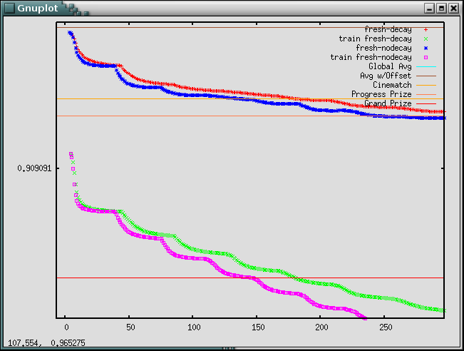
Here is the probe and training rmse for the first few features with and without the regularization term ("decay") enabled.
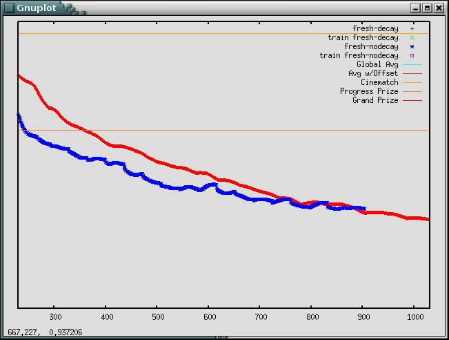
Same thing, just the probe set rmse, further along where you can see the regularized version pulling ahead:
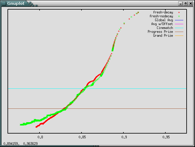
Same plot again, but this time showing probe rmse (vertical) against train rmse (horizontal). Note how the regularized version has better probe performance relative to the training performance:
Anyway, that's about it. I've tried a few other ideas over the last couple of weeks, including a couple of ways of using the date information, and while many of them have worked well up front, none held their advantage long enough to actually improve the final result.
If you notice any obvious errors or have reasonably quick suggestions for better notation or whatnot to make this explanation more clear, let me know. And of course, I'd love to hear what y'all are doing and how well it's working, whether it's improvements to the above or something completely different. Whatever you're willing to share,
-Simon